NumPy and OpenCV Exercises
If you get stuck, check back with the intro tutorials or ask the Vision Sublead or CSE.
Table of Contents
Getting Started
If you haven’t done this stuff to set up your environment, make sure to do so before getting started.
Installing Packages
Linux:
# pip install numpy
# python -m pip install numpy
# python3 -m pip install numpy
Windows:
# py -m pip install numpy
# py -m pip install scipy
# py -m pip install matplotlib
# py -m pip install opencv-python
Importing Packages
import numpy as np
import cv2
from matplotlib import pyplot as plt
from matplotlib import image as mpimg
from scipy.ndimage import convolve
Load an Image
img_name = mpimg.imread("filename")
Show an Image
plt.imshow(img_name)
plt.show()
or
cv2.imshow("Window Name", image_var)
cv2.waitKey(0)
cv2.destroyAllWindows()
Save an Image
plt.imsave(img_name, "filename")
Exercises
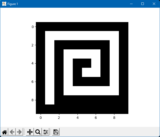
Exercise 1
Create and show/save a 10x10 spiral 1-bit image by modifying np.zeros() using only manual slicing operations (For help, see #3 of Intro to Computer Vision 1).
The completed image, when shown, should look like this:
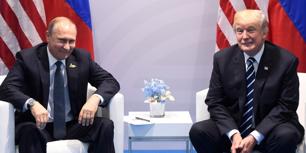
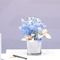
Exercise 2
Crop a square out of the “trump-putin.jpg” in such a way that we only see the flower in the center and no trace of either of the two people. Show/save this image. You must use array slicing operations. Don’t worry too much about getting it perfect, just make it so that we don’t see up to their black suits.
Starting Image:
One possible solution could look like this:
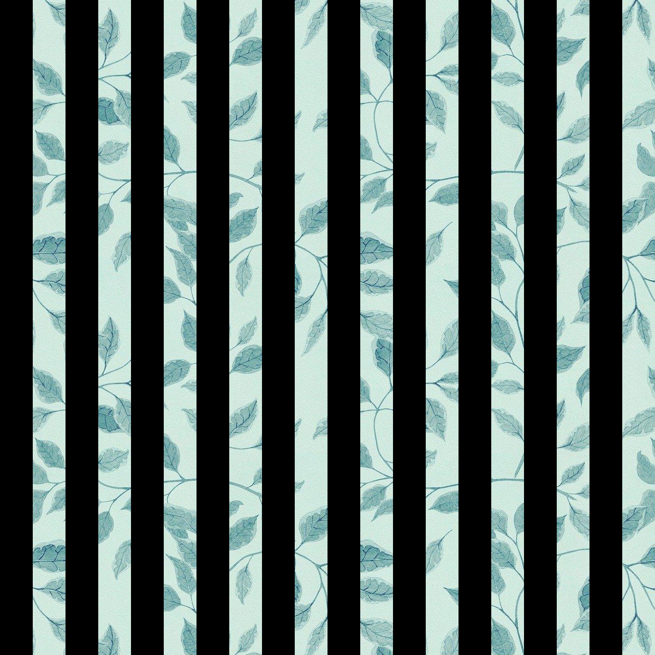
Exercise 3
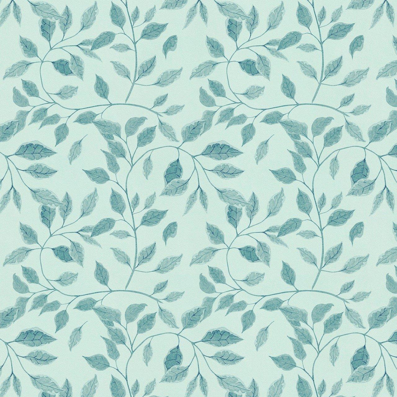
Combine “striped-leaf-pattern0.jpg” and “striped-leaf-pattern1.jpg” into one continuous leaf pattern image. Display/save this image. You must use np.where(). The core of this exercise (without the code for loading/showing/saving the images) can be done in a single line of code. (Don’t worry if the displayed image has purple stripes, the saved image should be correct).
Starting Images:

Here is what the solution should look like:
Exercise 4
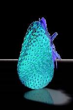
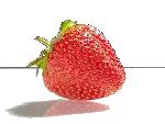
Consider “strawberry.jpg”. Figure out why the colors are messed up, and “squish” the image to make it look normal. Once done, remove as much of the black and white from this image (don’t worry about the shadow/reflection) such that there’s no more than 2 pixels of slack around the strawberry. Show/save the final image.
Starting Image:
One possible solution looks like this:
Exercise 5
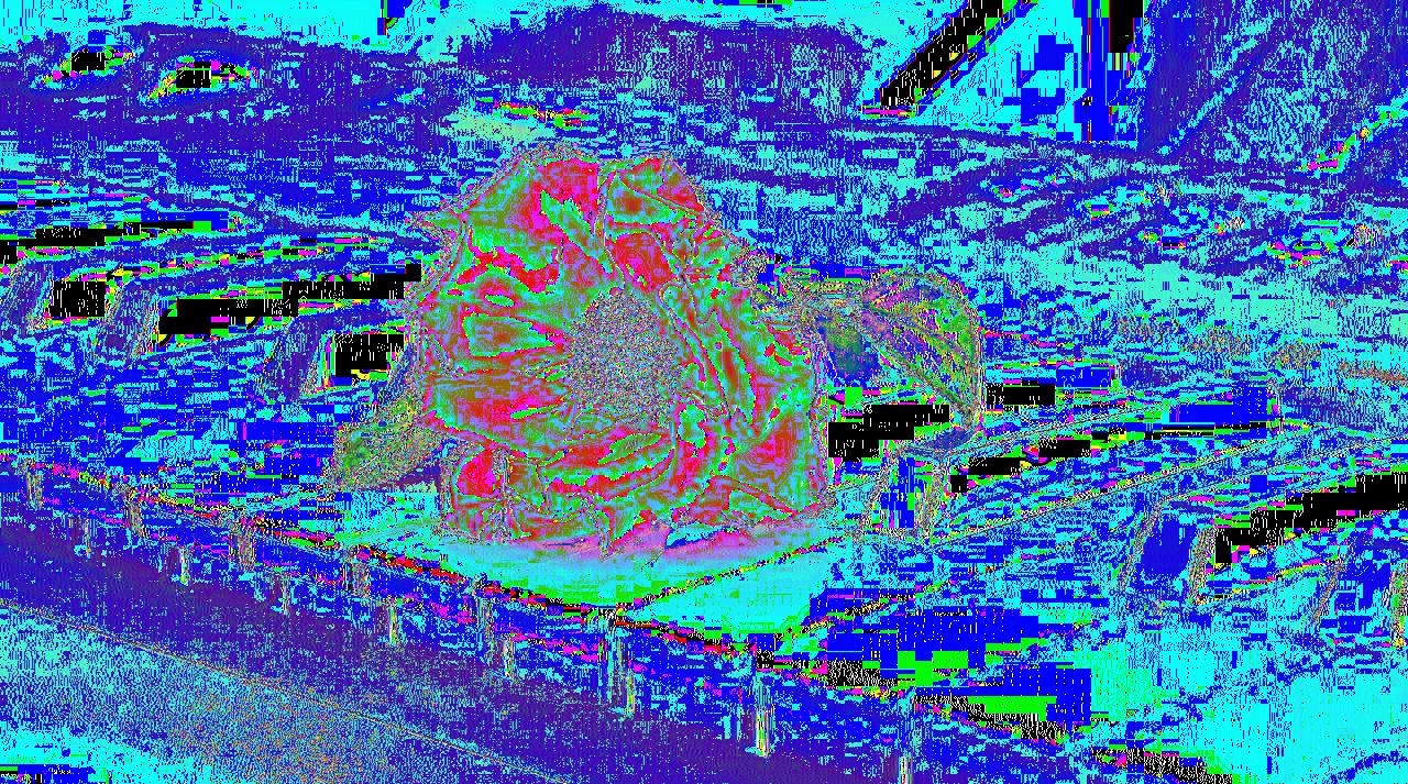
Consider “rose-piano.jpg”:

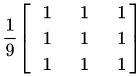
a) Apply blurring to “rose-piano.jpg” using image convolution with this normalized box blur kernel. You must use scipy’s convolve() function. Display/save this image.
One possible solution to part a looks like this:

- b) Repeat step a) but with a Gaussian blur using cv2.GaussianBlur() with a kernel size of (15, 15) and sigmaX=0. Display/save this image and compare with a). Click here for documentation on the cv2.GaussianBlur() function.
One possible solution to part b looks like this:

- c) Apply the following edge detection kernel to the regular image. You must use scipy’s convolve() function. Display/save this image.
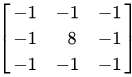
One possible solution to part c looks like this:
- d) Repeat step c) but use cv2.laplacian() with a desired depth of cv2.CV_8U and a kernel size of 3. Display/save and compare with c). Click here for documentation on the cv2.Laplacian() function.
One possible solution to part d looks like this:

- e) Repeat step d) but instead of using the normal image, use the Gaussian blurred image from step b). Display/save and compare with d).
One possible solution to part e looks like this:
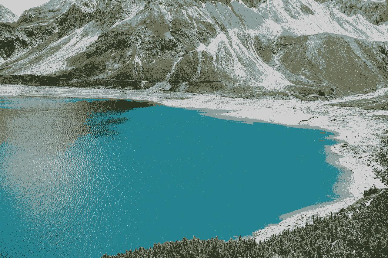
Exercise 6
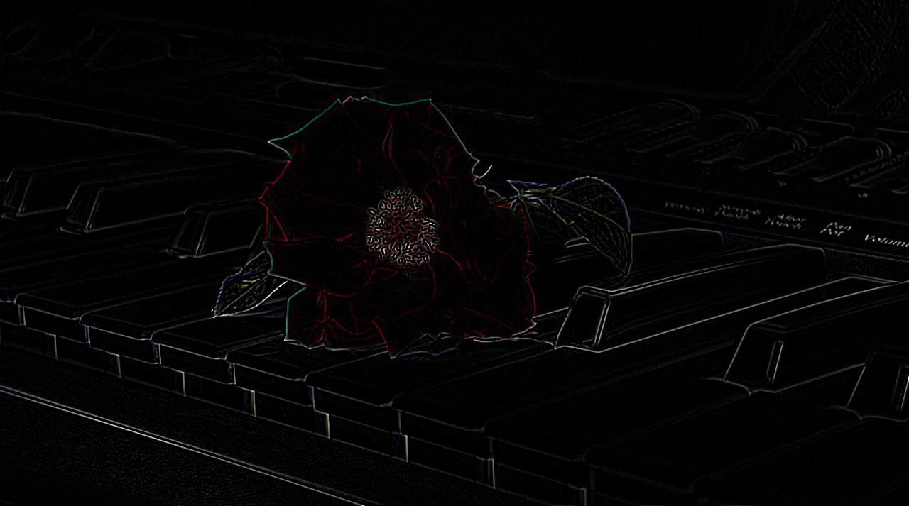
Apply k-means clustering to the “lake.jpg” image with varying kernel (K) sizes of 3, 5, and 7. Display/save the images from each kernel size. Refer to numbers 8-10 of the Introduction to Computer Vision 2.
Starting Image:

The clustered images should look like this:
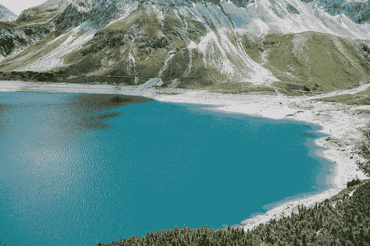
Download Image
Completed the exercises and want something more challenging? Check out the intro projects here.